Warning: package 'dplyr' was built under R version 4.2.3
Attaching package: 'dplyr'
The following objects are masked from 'package:stats':

    filter, lag
The following objects are masked from 'package:base':

    intersect, setdiff, setequal, union
library(tidyr)
Warning: package 'tidyr' was built under R version 4.2.3
library(ggplot2)
Warning: package 'ggplot2' was built under R version 4.2.3
# Read the dataset from a specified file pathdata =read.csv("E:/01-文件/04-UI文件/2401-【课程】BCB/BCB/BCB520Practice/data.csv")# Display the dataset in a nicely formatted table using knitr packageknitr::kable(data)
ENT
ID
YLD.2017.AB.Ran
YLD.2017.Soda.Ran
YLD.2017.Walla.Ran
52001
IDO854
91
45.0
71.0
52002
SRRN-6029
89
45.9
75.7
52003
SRRN-6028
84
40.9
75.3
52004
SRRN-6037
89
38.3
86.4
52005
LOUISE
90
52.6
75.9
52006
RIL29
89
43.7
59.0
52007
IDO629
81
45.8
72.2
52008
UC1110
95
45.5
88.0
52009
UC1642
90
49.3
80.9
52010
MT0921
85
38.6
78.1
52011
Choteau
89
51.4
84.0
52012
9223
88
56.8
84.9
52013
Attila-1RS
89
42.1
87.1
52014
Hahan-1RSMA
89
38.8
90.4
52015
10010/20
94
49.7
82.4
52016
MT0945
85
47.0
62.2
52017
Newana
82
45.9
88.3
52018
UC1682
88
42.7
59.0
52019
MT0813
91
51.9
65.4
52020
9229
83
45.5
87.9
52021
HW090006M
81
47.0
85.6
52022
H0800080
84
45.2
91.4
52023
H0800314
90
44.0
72.7
52024
MT1020
84
42.0
67.2
52025
9242
85
51.2
86.7
52026
Fortuna
96
51.6
71.8
52027
9260
87
46.7
59.2
52028
9232
93
51.1
41.5
52029
Tara2002
87
45.3
58.3
52030
UC1618
87
50.3
50.3
52031
9233
95
51.4
72.3
52032
WA8034
88
47.8
79.1
52033
IDO852
91
41.5
58.1
52034
IDO851
88
47.2
83.3
52035
WA8016
86
49.2
82.7
52036
IDO696
94
55.0
79.5
52037
28TH SAWSN-3045
92
43.9
68.4
52038
9247
93
41.7
85.8
52039
SRRN-6044
80
40.1
58.2
52040
9240
84
39.0
79.0
52041
Macon
102
44.6
74.9
52042
McNeal
88
41.5
61.6
52043
SRRN-6042
93
49.5
67.2
52044
RSI5 Yr5 Yr15 Gpc HMW 1
92
52.7
74.9
52045
Thatcher
91
48.6
80.8
52046
Jefferson
83
49.7
64.0
52047
IDO582
92
43.1
55.2
52048
IDO702
78
41.4
51.6
52049
IDO644
95
61.4
58.2
52050
WA8074
89
52.8
78.4
52051
IDO671
84
42.3
86.3
52052
SRRN-6099
85
52.8
63.1
52053
WA8123
82
47.5
63.6
52054
21TH HRWSN-2106
93
48.5
65.6
52055
H0800310
87
43.6
75.3
52056
H0900081
74
40.4
52.8
52057
Jerome
80
47.0
39.9
52058
Vida
87
42.7
60.9
52059
CENTENNIAL
94
43.2
51.8
52060
9252
93
41.9
60.6
52061
PENAWAWA
94
40.5
58.6
52062
UC1683
93
41.9
50.8
52063
Pomerelle
87
44.6
47.1
52064
MT1002
91
45.9
49.8
52065
Treasure
82
39.9
50.2
52066
Expresso
82
43.5
68.0
52067
HW080169
84
43.3
49.4
52068
Attila-1RSMA
84
45.9
57.2
52069
9259
95
48.6
55.8
52070
Cataldo
83
42.5
76.0
52071
11010-9, 10013-1
85
43.5
47.9
52072
9245
87
42.7
90.1
52073
SRRN-6049
88
42.8
49.6
52074
Kelse
93
45.1
62.0
52075
IDO687
94
48.0
85.1
52076
MT1053
87
41.7
92.7
52077
9256
84
47.2
54.9
52078
9253
99
43.7
50.0
52079
IDO560
87
42.8
38.6
52080
Alturas
93
40.5
77.5
52081
UC1551
91
53.6
85.4
52082
UC1554
76
45.9
78.0
52083
SRRN-6050
88
38.9
46.4
52084
IDO858
92
42.0
53.1
52085
UC1396
90
39.4
38.9
52086
PI610750
90
47.8
95.1
52087
Hollis
94
39.0
54.4
52088
LCS Atomo
82
39.9
37.5
52089
UC1395
84
40.4
48.5
52090
9241
91
42.0
47.9
52091
UC1603
83
39.9
49.4
52092
UI Winchester
85
45.1
36.2
52093
UC1601
78
44.1
43.8
52094
WA8099
80
40.5
74.8
52095
CAP151-3
82
48.7
44.6
52096
MT0415
83
46.5
61.2
52097
WHITEBIRD
86
47.5
80.9
52098
21TH HRWSN-2126
84
43.4
52.0
52099
LCS-Star
78
41.9
69.3
52100
Scarlet
80
37.9
55.2
52101
UC1552
83
39.5
74.6
52102
Jubilee
88
44.7
70.5
52103
SRRN-6032
86
44.4
54.0
52104
Otis
87
53.6
87.9
52105
IDO488
81
42.1
60.5
52106
SRRN-6019
83
51.9
57.6
52107
SRRN-6047
86
39.2
55.3
52108
MT1016
91
41.5
50.8
52109
Hahan-1RS
86
42.8
59.7
52110
MTHW1060
82
45.6
54.0
52111
SpCB-3004
84
41.3
63.2
52112
SY Capstone(IDO694?)
87
40.0
66.6
52113
UC1643
92
42.1
55.0
52114
9246
86
40.4
72.9
52115
chewink
80
48.0
78.1
52116
MTHW0771
87
40.5
54.5
52117
H0900009
84
45.3
52.9
52118
9225
83
46.1
56.6
52119
9254
87
43.0
45.7
52120
10014/7
93
40.1
77.2
52121
Lassik
80
40.4
62.1
52122
Summit 515
89
39.0
67.8
52123
MT0861
95
48.2
57.6
52124
9249
94
52.2
53.2
52125
Lolo
90
51.9
56.6
52126
RIL203
93
52.0
58.7
52127
MT1027
92
46.0
67.3
52128
UC1616
94
44.6
47.5
52129
UI Stone
95
40.5
69.3
52130
UI Pettit
92
42.0
55.0
52131
28TH SAWSN-3046
92
40.7
53.4
52132
WA8133
85
42.5
82.5
52133
SRRN-6109
88
49.0
43.0
52134
UC1602
87
46.1
75.1
52135
9228
92
44.6
64.2
52136
21TH HRWSN-2111
89
43.6
54.1
52137
Hi-Line
80
38.8
57.9
52138
AC BARRIE
86
42.9
49.6
52139
H0800103L
81
39.4
77.3
52140
IDO868
94
44.8
63.8
52141
UC1679
86
42.0
59.6
52142
9248
85
39.0
46.6
52143
WA8100
81
44.9
53.2
52144
MTHW0867
92
47.8
55.5
52145
9258
87
47.5
60.1
52146
IDO440
89
38.3
65.2
52147
Duclair
92
45.3
49.6
52148
UC896 5+10 Lr34/Yr18 Yr5 Gpc
89
38.8
48.2
52149
Blanca Grande 515
89
37.1
52.7
52150
9263
86
45.4
49.3
52151
SRRN-6098
93
48.8
54.6
52152
9261
80
37.6
76.2
52153
SRRN-6097
90
42.2
85.8
52154
9262
94
39.5
58.4
52155
SRRN-6030
96
38.0
76.2
52156
HR07024-5
95
37.8
54.1
52157
UI Lochsa
99
41.5
65.2
52158
CAP34-1
94
45.5
53.4
52159
HW090071M
93
46.1
65.1
52160
UC1599
80
38.8
63.2
52161
MTHW1069
87
45.9
67.4
52162
UI Platinum
96
50.0
62.1
52163
Blanca Fuerte
91
46.8
52.4
52164
Berkut
87
45.8
57.9
52165
SRRN-6027
88
43.2
51.0
52166
IDO686
91
47.1
61.3
52167
SRRN-6038
81
38.1
69.3
52168
HR07005-3
82
43.7
62.5
52169
IDO377s
85
47.2
59.3
52170
MT0802
92
39.9
64.3
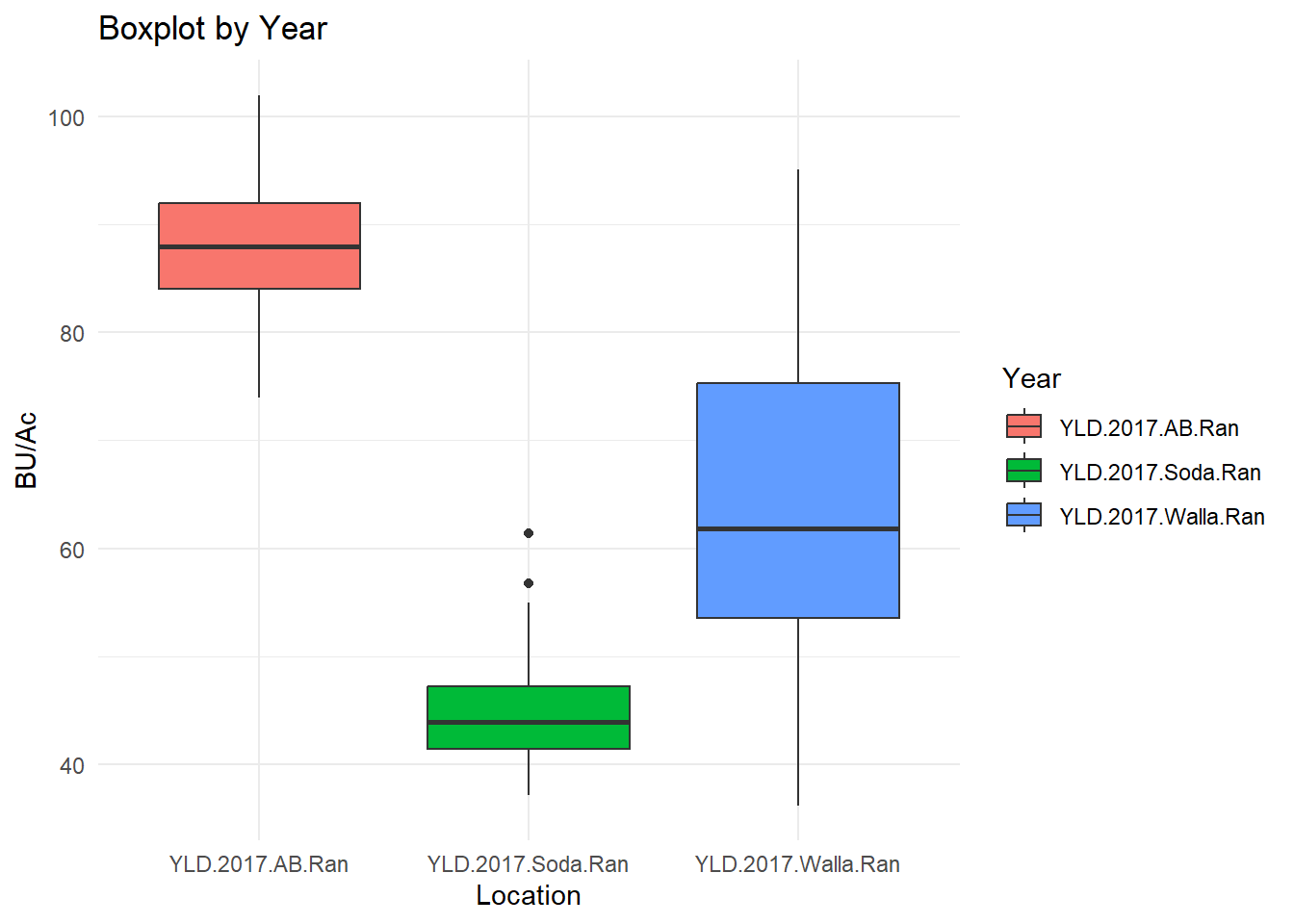
# Transform data from wide to long formatlong_data <- data %>%pivot_longer(cols =starts_with("YLD"), # Select columns that start with 'YLD'names_to ="Year_Rep", # New column for yearvalues_to ="Value"# New column for values )# Extract the year from 'Year_Rep' and create a new column 'Year'long_data <- long_data %>%mutate(Year =sub("-.*", "", Year_Rep)) ggplot(data=long_data, aes(x=Year, y=Value, fill=Year)) +geom_boxplot() +# Add boxplot layertheme_minimal() +# Use a minimal themelabs(title="Boxplot by Year", x="Location", y="BU/Ac") # Add labels
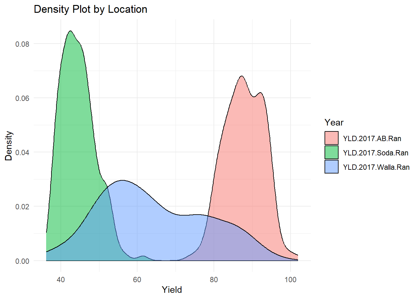
# Create a density plot of 'Value' by 'Year'ggplot(data=long_data, aes(x=Value, fill=Year)) +geom_density(alpha=0.5) +# Add density layer with transparencytheme_minimal() +# Use a minimal themelabs(title="Density Plot by Location", x="Yield", y="Density") # Add labels
Describe
The dataset comprises a 2D table format, focusing on wheat as the primary item. It includes three distinct attributes: Order, YLD-2017-AB-Ran, YLD-2017-Soda-Ran, and YLD-2017-Walla-Ran, each with 170 items.
Order: This attribute is ordinal and sequential in nature. It represents a series of 170 unique identifiers for the data entries.
YLD-2017-AB-Ran: This quantitative attribute reflects a range of values between 73.8 and 101.9. It is associated with the geographical coordinates of 42.96° N latitude and 112.83° W longitude, which corresponds to the AB region.
YLD-2017-Soda-Ran: Another quantitative attribute, it spans a range from 37.1 to 61.4. The Soda region, located at 42.6544° N latitude and 111.6047° W longitude, is the geographical reference for this attribute.
YLD-2017-Walla-Ran: Similar to the other YLD attributes, this is also quantitative, with a range of 36.2 to 95.1. It is linked to the Walla region, situated at 46.0646° N latitude and 118.3430° W longitude.
TASK ABSTRACTION
Discover Outliers where production data exists within the same location;
Compare the distribution of data across different locations.